Excel for GIS: Basics 1

If you're like me, you may be happily plugging along in your GIS career for quite some time before you need to use Microsoft Excel beyond the basics. But the day may come when you find yourself on a multidisciplinary team with the need to work with people in other disciplines.

Moving data back and forth between your GIS software and Excel may get tiresome. And it may be that you decide that the best thing to do is to learn how to do some of the tasks you are used to doing in GIS, in Excel.

If so, this blog is for you. The plan is to save you some time by having much of what you need to know in one spot. This blog is Part 1 of a series.

Basics 1

Relational and absolute cell references

You have no doubt noticed that Excel reads your formulas in a relational fashion. That is, when you copy a cell that contains a formula, the formula references shift with the new data location.

For example, the cell with the formula shown below was copied from the one above it. If you clicked on the cell above, it would read =D2-C2.

But what if you don’t want the formula references to move with the cell? An absolute cell reference is written with dollar signs before the row and column references.

For example, the cell with the formula shown below was also copied from the one above it, but the absolute cell reference is repeated without any shifting. If you clicked on the cell above, it would also read =$B$14.

 

Named Ranges

Simply put, a named range is a block of cells that can be referenced by a name that you give it.  

How to make a named range

To create a named range: 1) select the block of cells you want to name—then with the cells still selected—2) type the name in the name box.

The example below shows how to create a named range for a single cell.

And this example shows how to create a named range for a block of cells.

How to reference a named range

Use the range name in any formula in place of a range of cells.

The example below shows how to reference a single cell.

Below is shown an example of referencing a block of cells.

Table objects

A table object in Excel looks similar to a formatted block of cells that a user might call a table. But it has additional functionality that will make your work easier. 

Note that I will often show range references in formulas for this blog as they appear in reference to Tables.

Removing table objects

One caveat to table objects is that not all import programs in other software recognize them. You may find other reasons why you want to use a normal range instead of a table after you have already created the table. If you run into this, right-click anywhere on the table and select Table > Convert to Range. Note that this does not transform the table into a named range. You will need to reselect the block and rename it if you want to use what was the table as a named range.

How to create a table object

The steps to create a table are shown below: 1) Highlight your table; 2) Click Home – Format as Table (drop down arrow); 3) Select a style from the drop-down.

When you click on the style above, the dialog below will pop up. Make sure the header checkbox is set correctly and click OK.

Following the above instructions, your finished table should look something like the one shown below.

By default, each column will have auto filters , and the table will have a blue color scheme (you don’t have to choose a style like we did).

To see other options, click anywhere in the table, and click the Table Tools Design tab. To change the table name, fill in the Table Name box (see below). It is good practice to change the name to something easy to use, in the same way you would choose a range name.

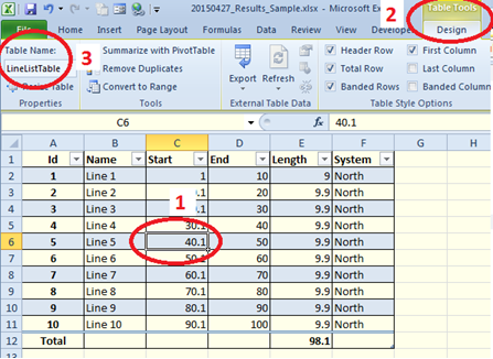
Note that I have also checked the Total Row checkbox, so I can add a total for the Length column; and I have also checked the First Column checkbox, so that the first column becomes bolded.

(Continued in next blog of this series)