If you're like me, you may be happily plugging along in your
GIS career for quite some time before you need to use Microsoft Excel beyond
the basics. But the day may come when you find yourself on a multidisciplinary
team with the need to work with people in other disciplines.
If you're like me, you may be happily plugging along in your
GIS career for quite some time before you need to use Microsoft Excel beyond
the basics. But the day may come when you find yourself on a multidisciplinary
team with the need to work with people in other disciplines.
Moving data back and forth between your GIS software and
Excel may get tiresome. And it may be that you decide that the best thing to do
is to learn how to do some of the tasks you are used to doing in GIS, in Excel.
If so, this blog is for you. The plan is to save you some
time by having much of what you need to know in one spot. This blog is Part 2
of a series.
Basics 2
How to reference cells and ranges in a table object
Single Cell In Current Row. To reference a cell in the
same row, put a @ sign before the column name and enclose the entire column
name in brackets, as shown below. The formula shown below is the same as E3 =
D3-C3.

Calculated Columns.
Note in the example below that the entire table column is filled with
the formula by default. You are also presented immediately with a drop down
with a choice to Undo Calculated Column.
If you click Undo Calculated Column,
your formula will only apply to the active cell. If the formula has overwritten
existing formulas in other rows, and you click Undo Calculated Column, all the formulas are undone except the
active cell, i.e. your data will not be ruined.
Single Column. To
reference a single column of a table, put the table name followed by the column
name in brackets if the column is in a different table from the active cell, as
shown below.

Note that if the column is in the same table as the active
cell, the table name is left off, as shown below.
=MAX([Length])
Multiple Columns.
To reference a multiple columns of a table, put the table name followed
by the column names in brackets in the format first column:last column, as
shown below. This formula is saying to get the maximum value contained in the
columns with headers 2009, 2010, 2011, 2012, 1013, and 2014.

Unlike the single column reference, if the active cell is in
the same table as the referenced columns, the table name is still needed.
Also, you can use noncontiguous ranges, but you will need to
type in the cell references the normal way.
Maintaining Column Types And Precision
It is as important to specify column types in Excel as in
GIS or database software, for the same reasons. For example, if you don’t
specify a column containing a value such as “007” as text, it may be read by
Excel as “7”. If you have many records, as we often do in GIS, it is not an
easy or quick task to get values back to where they were once they have been
accidentally changed.
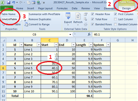
Visible and actual values
Note that—because of column formatting—the values you see on
your screen may not be what is in the cell.
See the image below for an example. The column is formatted to show only
2 decimal places, but the actual value has many more. This can cause problems
of various sorts. If you want to create actual numbers limited to a certain
precision, create a new column and use the ROUND function to calculate in
rounded values. Using the spreadsheet below, the formula would be
=ROUND([@MP2], 2)

Invisible characters
Sometimes you will find functions that require matching
values don’t work for inexplicable reasons, for example, functions like VLOOKUP
and MATCH. Upon further examination, sometimes you will find things like
leading or trailing spaces, sometimes you may not be able to figure it out. In
any case, it may not be practical to fix the problems one by one by editing the
cells. Something to try is to to trim and clean the values.
The TRIM function trims leading and trailing spaces from
cells. The CLEAN function removes 31 non-printing characters that can exist in
Excel (not spaces). Since the two functions remove different characters, it
does not matter what order you perform them, and you can combine them, as
follows:
=TRIM(CLEAN(B12))
Unique Values
To make a list of the unique values in a column (or any
selection), use Data > Remove
Duplicates.
The first step is to make a copy of the data that you want
to find unique values for. This is necessary because the duplicates are removed
in-place. Your copy will become your list of unique values. The first step is
shown below, where the PipeSysNam
column is copied to the right of the table.

Next: 1) Leave the copied selection selected; 2) Click the Data tab; 3) Click Remove Duplicates; and 4) Fill out the Remove Duplicates dialog—headers and columns to use—and click OK.

When you click OK
on the Remove Duplicates dialog, a
message will appear informing you of how many duplicate values were removed and
how many unique values remain. Click OK.

If you use multiple columns, the tool finds unique values
across all columns.
You can do something similar by using the Data > Filter > Advanced tool.
Highlight the range you want to filter, open the tool, then specify Copy to another location and Unique records only. See the image below.

Parsing text
To parse a text column into multiple
columns, use Data > Text to
Columns. The first step is: 1) Select the column or block to parse;
2) Click the Data tab; and 3) Click
the Text to Columns tool. This will
bring up the Convert Text to Columns
Wizard dialog.

The Wizard
consists of 3 steps. In Step 1,
select the radio button to indicate whether your data is delimited or fixed
width. Click Next when you are
finished.

The next two images both show Step 2, the difference being
whether “Delimited” or “Fixed Width” was chosen as the data type.
In Step 2 with
delimited data, choose your delimiters, whether to treat consecutive
delimiters as one and define a text qualifier. Typically, you will only need to
pick your delimiters on this step and take the default settings for the rest.
Scroll down the Data preview pane to
see how your choices affect the result. Click Next when you are finished.

In Step 2 with fixed
width, set your column breaks, whether to treat consecutive delimiters as
one and define a text qualifier. Typically, you will only need to set your
column breaks on this step and take the default settings for the rest. Scroll
down the Data preview pane to see how
your choices affect the result. Click Next
when you are finished.

The image below shows how our example looks after being
parsed by this tool. Note that if I had specified that the columns were text,
the “0” in Cell X3 would have been maintained as “00” if that is what I had
wanted.

There are more advanced ways to parse text using formulas
and VBA scripts, but this is by far the simplest way until you get to that
point.
Concatenating columns
Concatenate columns with the CONCATENATE formula, as shown
below. Note that the pieces of the concatenated value are comma-delimited, and
the parts can be columns, text or formulas.

Special Paste
Transposing Columns and Rows
Transpose columns to rows or rows to columns with the Special Paste function. 1) Select the
range to copy, 2) right-click the destination cell and 3) select Special Paste > Transpose, as shown
below.
Before

Transposed

Values
To copy/paste only the values from a range derived from
formulas/functions or a range that is formatted, use the Special Paste function. Select the range to copy, right-click the
destination cell and select Special Paste
> Values.
This function is useful to speed up your workbook. Too many
formulas to re-calculate can cause your workbook to work slowly, and you may
not want to turn off automatic formula calculation. An easy way to remove
formulas is to copy a range with formulas, then Special Paste > Values back onto itself (don’t move the cursor).
This function is also useful to maintain the integrity of
your data if someone else will be using your workbook. They may accidentally
delete the data behind formulas (or you may forget and do the same thing!). As
above, copy the range onto itself, using Special
Paste > Values, to remove the formulas or links.
Paste Link
To create links from a copied range to a range pasted into,
use the Special Paste function.
Select the range to create links for, right-click the destination cell and
select Special Paste > Paste Links.
The image below shows the user has copied Cell E14, then
used Special Paste > Paste Links
to paste a link from Cell E14 into Cell C24.
Note that Cell C24 is selected, and the input box shows the
link just pasted in from Cell E14. Note that this function creates absolute
references.

This function doesn’t work in Tables, but does work in named
ranges or normal cells
Filter by selected cell
Filter quickly by highlighting a range containing what you
want to filter on, right-click, and choose your filter choice, as shown below. Note
that you can filter by text color or background color, as well as values.

(Continued in the next blog of this series.)